The standard, protocols, and quality-assurance procedures used to hand-annotate
the field boundaries that trained the Trazo models. It covers how a field is
defined, how boundaries are drawn, the decision rules for ambiguous cases, and
how the annotation procedure itself was validated against ground truth and across annotators.
Adapted from the Trazo technical note (Grupp et al. 2026), Methodology and Appendix A · Read the full note
1 Definition
What is a field?
At the core of these guidelines is a single, shared definition of an agricultural field.
Our definition
A field is a clearly bounded land unit that is actively or recently managed. It is visibly distinct from natural vegetation across multiple time periods and is used in the production of crops, pasture, or other consumable goods. Fields may incorporate some natural features if those features have been subsumed into the production process. Areas overtaken by regrowth, or lacking signs of management, are not included.
A field includes farms, pastures with discernible management, and plantations of tree crops whose pattern is distinguishable in Sentinel-2 imagery.
In manual annotation, the goal is to delineate the idealized boundaries of such fields, in the manner we would want an AI model to automatically delineate them.
Boundaries are produced without concern for crop type. While annotating in the Chiquitania and Mato Grosso, it proved nearly impossible to reliably differentiate among annual crops, and even pasture or cover crops were often hard to separate from annual crops, by visual inspection, even with temporally coincident very-high-resolution imagery. We therefore took a field-inclusive approach: annotators trace every field that shows clear signs of human management.
2 Method
The annotation approach
Annotators trace digital field boundaries on each Sentinel-2 chip, using Planet Labs basemaps as a reference.
Use multi-temporal imagery
Always view at least two Sentinel-2 time windows, typically the start and end of the growing season, and align them with Planet Labs monthly basemaps from the same year. Comparing time windows improves boundary clarity and avoids mislabeling mid-harvest fields.
Annotate the whole field, even beyond the chip
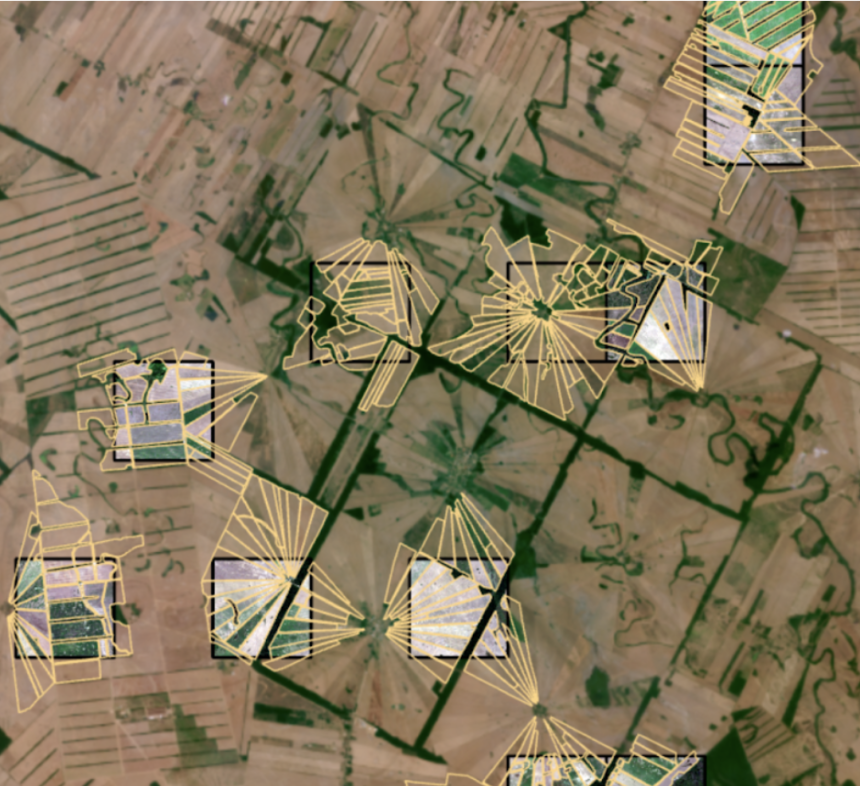
Annotate every field, and the entirety of each field, even if only part of it falls inside the chip (Figure 1a). Capturing the complete boundary, rather than just the portion inside the chip, preserves flexibility for downstream applications and gives an unbiased estimate of field size.
Draw at the visual edge, including mixed pixels
Boundaries should be placed at the visual edge of the field, even where this includes "mixed pixels" that blur the interior and exterior. This ambiguity is important for model learning, because real-world boundaries are rarely crisp.
Zoom out for context
Periodically zoom out to understand the broader landscape. This clarifies whether a patch is part of a managed system or natural regrowth, and avoids creating unnecessary boundaries from subtle color variations seen when inspecting too closely.
Distinguish managed from natural vegetation
Annotate fields with visible boundaries, distinct textures, and signs of active management, even when fallow. This matters especially in regions like the Amazon, where shifting cultivation is common. Tree crowns arranged in rows or other planting structure indicate management. Do not annotate dense regrowth, contiguous natural tree crowns, or randomly distributed vegetation. Label pastures only where there are clear signs of clearing or maintenance.
The two figures below show the core protocol. Click any figure to enlarge it.
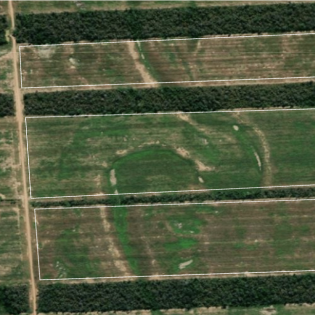
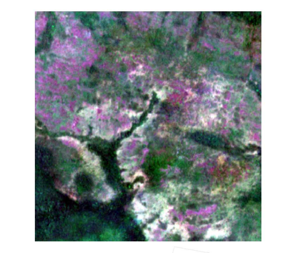
Figure 1a. Example fields overlaying sampled chips annotated in the Chiquitania ecoregion. Both the Sentinel-2 chip (model input) and temporally coincident Planet Labs basemaps (annotation reference) are visible. Fields are annotated completely even where they extend outside the chip.Figure 1b. Natural vegetation can be subsumed into the field or serve as a border. A useful decision rule: "If you were standing in the middle of the field and this feature was in front of you, could you cross it on foot?"
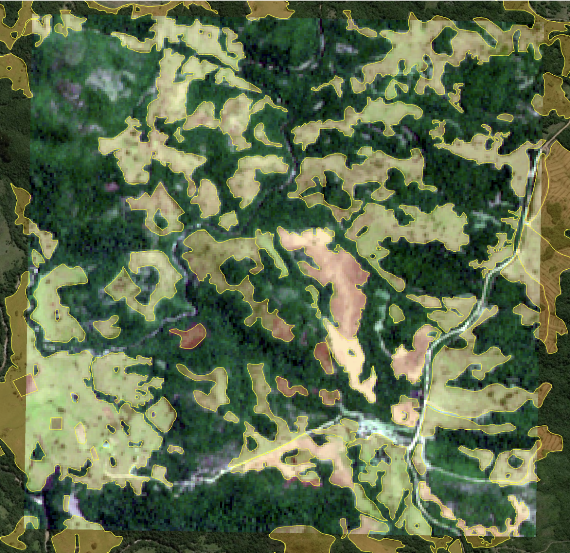
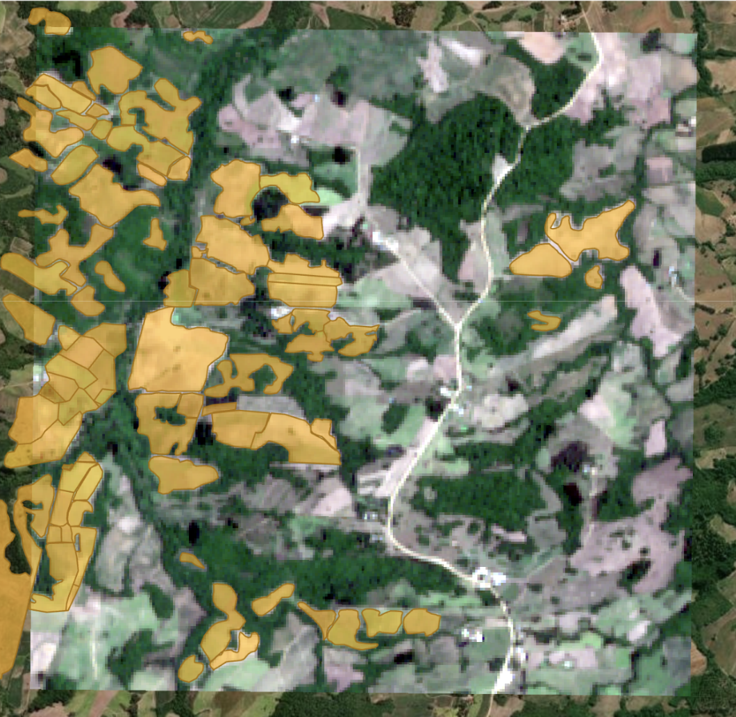
Figure 1c. A fully labeled chip in the Uruguayan Savannah; the pale polygons are entirely labeled fields.Figure 1d. A chip in the Uruguayan Savannah with fields partially completed by an annotator, showing the process. This chip contains mixed pasture and annual crops; separating annual crops from pasture is, in many contexts, impossible from the annotator's perspective.
3 Guidelines
Complete annotation guidelines
The full set of guidelines for manually annotating field boundaries.
Use of multi-temporal imagery: always visualize at least two Sentinel-2 time windows and align them with Planet Labs monthly basemaps from the same year. This improves boundary clarity and avoids mislabeling mid-harvest fields.
Boundary drawing: draw boundaries at their actual visual edges, even through "mixed pixels." This ambiguity is helpful for model learning.
Keep the area as one field if interior and boundary pixels are highly intermixed.
Split the area only if there is a visibly clear divide and at least 1 to 2 pixels of pure, unmixed interior.
Label beyond chip extent: always label the entire field, even if it extends past the chip boundaries, to allow flexibility for future resizing or merging.
Contextual zooming: zoom out regularly to better discern field shapes and surrounding land-use patterns, which often resolve more clearly at broader scales.
Shifting agriculture and pasture: use a splitting technique, drawing the overall agricultural extent and then splitting it into plots, when fields touch or have ambiguous shapes, especially in dense zones.
Soft boundaries: leverage the NIR composite in Sentinel-2 to detect subtle differences between adjacent field interiors or soft edges.
Background definition: background is characterized by a lack of change over time, or static exposed soil. These should not be labeled as fields.
Plantations: tree crowns arranged in rows often signal active management, so label them as fields. Randomly dispersed crowns suggest natural regrowth, so do not label them.
Inclusion criteria:
Include fields even if they are fallow or inactive. This is especially important in shifting-agriculture contexts such as the Amazon.
Include fields in the later time period created from the conversion of nature (Figure 2).
Include pasture only if it shows clear signs of human intervention or vegetation clearing.
Include small stands of native vegetation within a field if they are part of the managed unit and not forming an edge.
Include natural features such as creeks if they have been drained, modified, or clearly integrated into the managed field.
Exclusion criteria:
Do not label patches where regrowth or natural vegetation has overtaken the land.
Do not label fields that have transitioned to secondary forest, or where vegetation shows a random tree distribution.
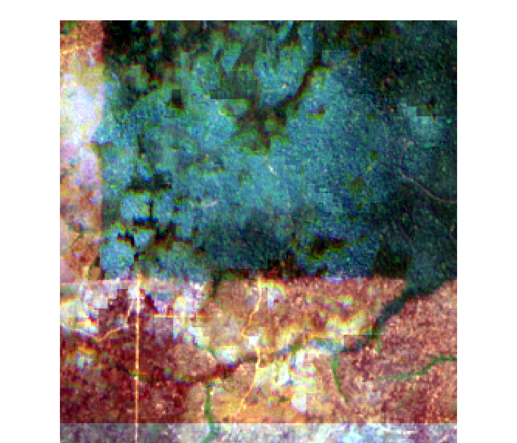
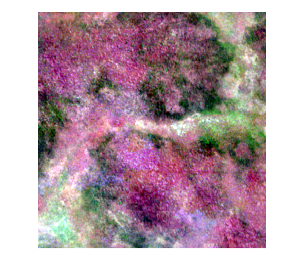
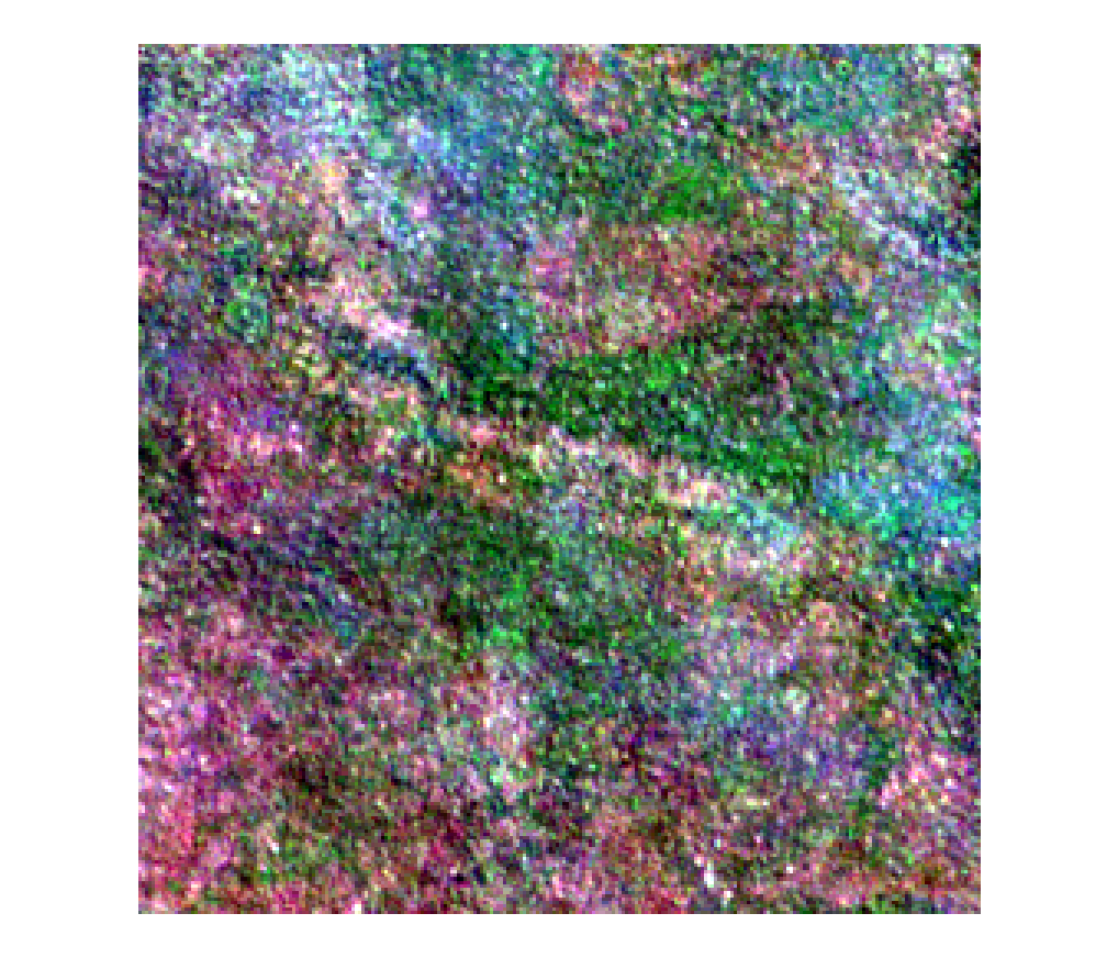
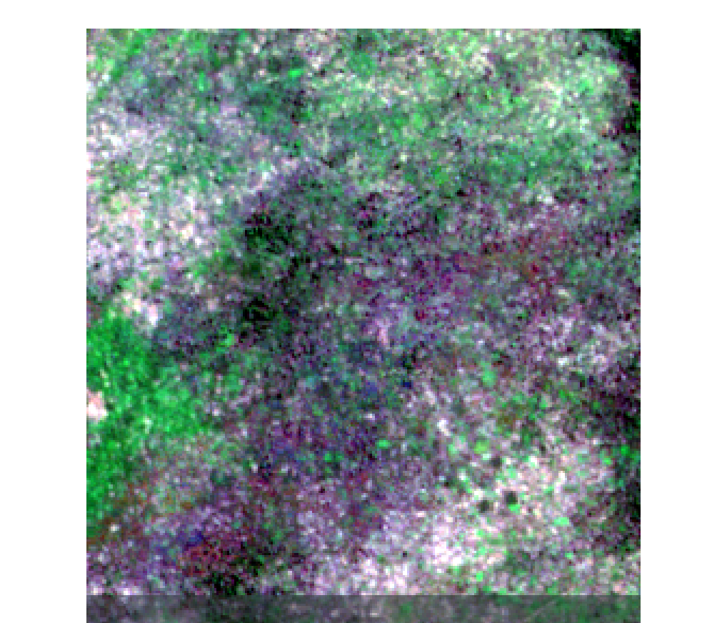
Avoid labeling burned areas unless there are clear signs of structured management such as rows or regularity (Figure 3).
For wetlands converted to agriculture, remove low-lying features only where they contain standing water, which stands out in the NIR band.
Exclude buildings if they lie at or near the field boundary.
When unsure whether to label a field, ask:
Is there a clear visual boundary?
Is the patch distinct from natural vegetation?
Does the area appear actively managed, or is it transitioning back to nature?
If an end user saw this area left unlabeled, would it appear to be a mistake?
These protocols were continually refined and augmented throughout the labeling effort to improve consistency and accuracy, with the aim of producing boundaries that are clear, reproducible, and useful to downstream users.
4 Edge cases
Decision rules for ambiguous cases
Additional decision points specified to guide consistent calls on the hard cases.
If interior and boundary pixels are highly intermixed, keep the area as one field unless there is a clear visual divide and at least 1 to 2 pixels of unmixed "pure interior."
Features like creeks are part of a field only if they have been drained or clearly integrated into management; otherwise they form boundaries (Figure 1b).
Buildings at the edge of a field are excluded from the label.
Exposed soil, or areas with little to no change over time, should not be labeled, as they likely represent background or barren ground.
In general, prioritize inclusivity over exclusivity: if a field has a clear boundary and is visually distinct from surrounding natural areas, consider it for annotation. Our guiding principle was framed this way: "Imagine an end user is viewing the final product of field boundaries generated by Trazo models. Looking at the candidate field you are considering, if its absence in the final product would be perceived as an omission error by the end user, then annotate the field."
Conversely, if the land appears unmanaged, managed for non-cultivation purposes such as urban development, naturally disturbed, or in the process of returning to forest, it should be excluded.
5 Quality assurance
Peer review & quality assurance
Every field boundary annotation passed through three rounds of peer review.
Group discussion and consensus: weekly meetings with project researchers and annotators discussed difficult examples, reached consensus on how each should be labeled, and updated the protocols to cover similar future cases.
Cross-annotator evaluation: when an annotator completed a task, other annotators reviewed the work for consistency and accuracy.
Manager evaluation: a project data scientist reviewed the final set of annotations from every annotator to ensure accuracy and consistency across the team.
Consensus labeling and quality assurance are key to accelerating performance gains in model development, especially for active learning, where informative but challenging samples are selected for targeted annotation (Estes et al. 2022). Newly onboarded annotators always label the calibration set first, before contributing to the corpus.
6 Conversion
Recent conversion & burned areas
Critical to the EUDR use case is delineating recently converted fields and the practices that cause conversion.
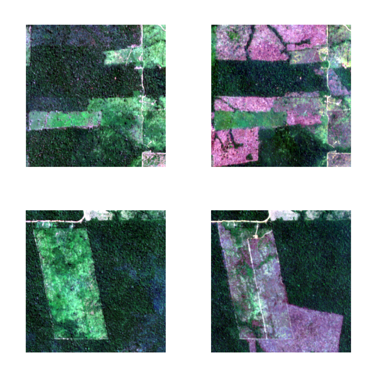
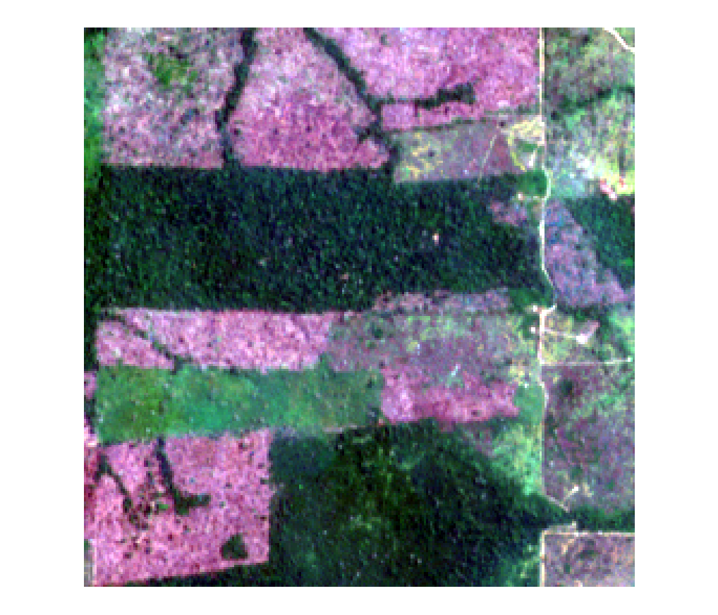
Annotators include fields present in the later time period that were created by the conversion of nature between the planting and harvest windows. These recent conversions are annotated when they have a discernible management pattern and can be represented as a field object, even though they are absent from the earlier window. Trazo models thereby encode recent conversion.
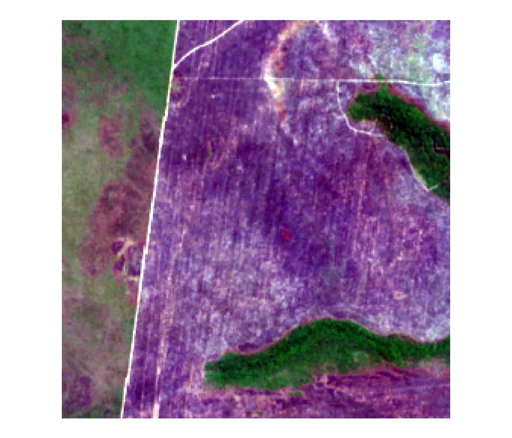
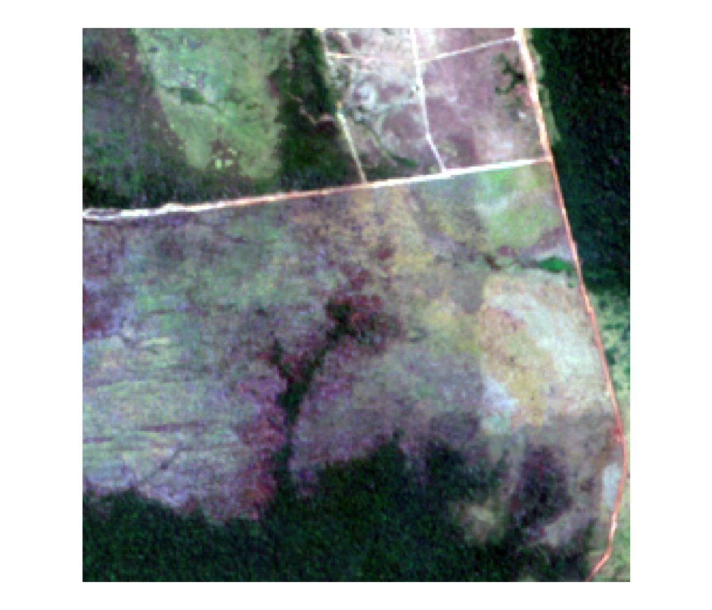
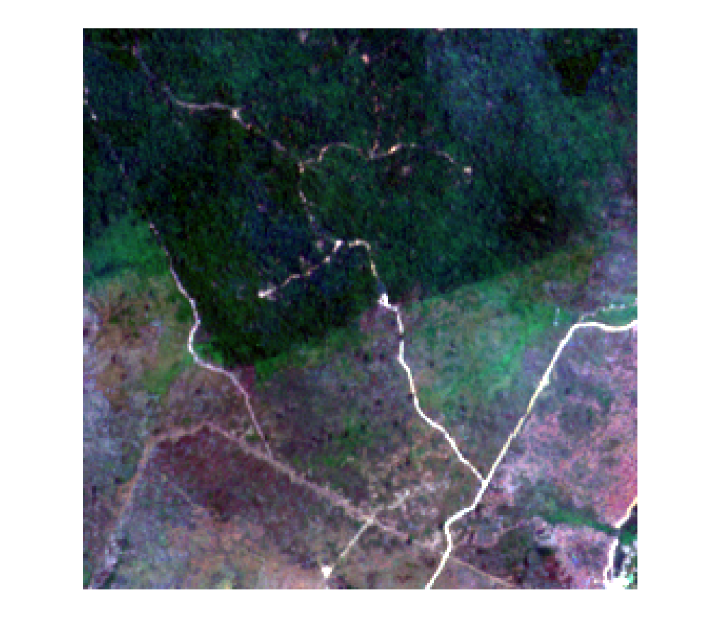
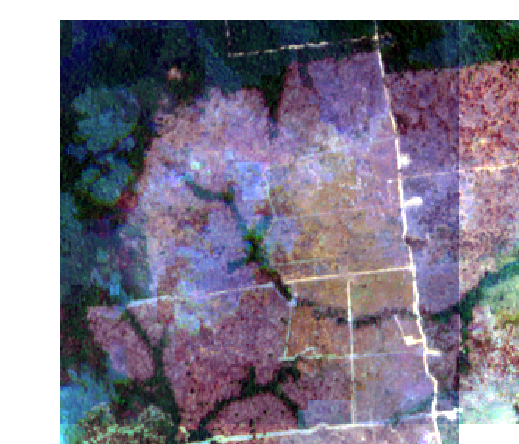
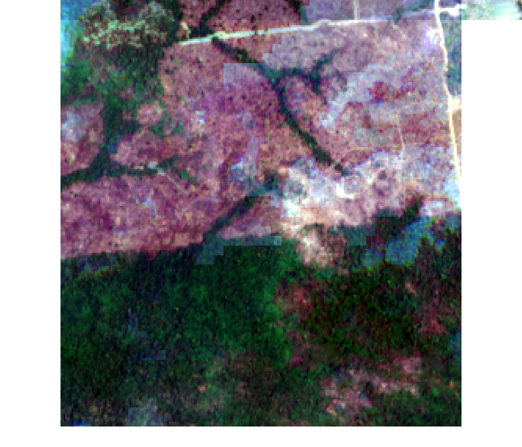
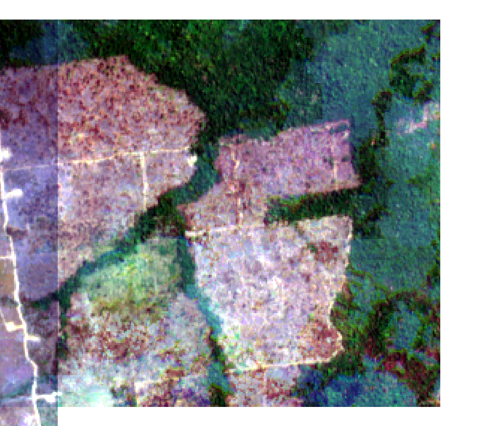
Figure 2. Samples where conversion occurred between the two time windows. Row 1: two chips from the same area and year, one in planting and one in harvest, from the Mato Grosso low-confidence active-learning set. In the harvest season, new fields were opened by burning, visible as pink burn scars; these are labeled despite their absence in the earlier window. Row 2: a second example. Recent conversions are annotated when they show a discernible management pattern. Imagery: Sentinel-2.
Burned areas
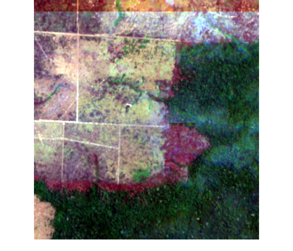
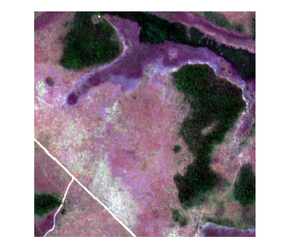
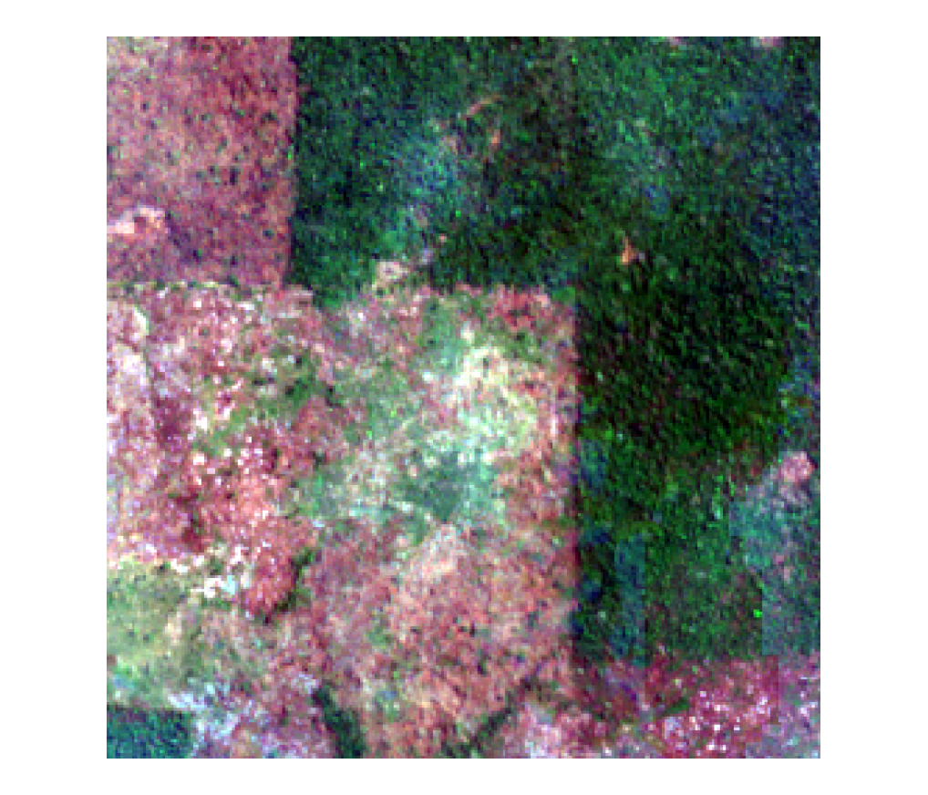
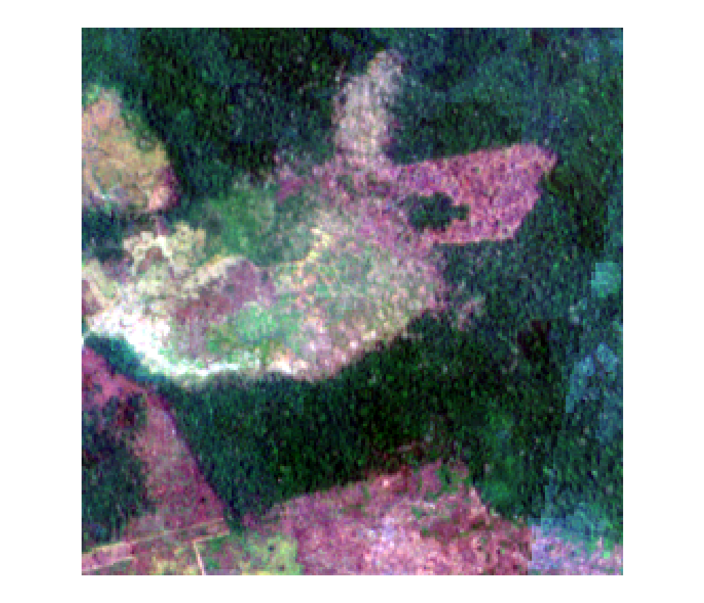
Burned areas are labeled only when they show human-induced regularity, such as burning in rows or other structured management. Burn scars without a distinguishable, managed object are not annotated. Each panel below cycles through four example chips.
Figure 3b. Burn pattern with vegetation recovering. These were annotated.
Figure 3c. Burning with haze from clouds and fires. These were annotated.
Figure 3d. Burning without a clear pattern. Not annotated.
Figure 3. Examples of regularized burning versus burning without distinguishable objects. Imagery: Sentinel-2.
7 Scope
Agricultural classes
The field-inclusive approach corresponds to the following MapBiomas classes treated as agriculture.
Table A-1. MapBiomas classes included in the agricultural class
Code
Class (English)
Group
9
Forest plantation
Silvicultura
15
Pasture
Pastagem
20
Sugar cane
Cana
21
Mosaic of uses
Mosaico de usos
35
Palm oil
Dendê
39
Soybean
Soja
40
Rice
Arroz
41
Other temporary crops
Outras lavouras temporárias
46
Coffee
Café
47
Citrus
Citrus
48
Other perennial crops
Outras lavouras perenes
62
Cotton (beta)
Algodão (beta)
8 Validation
Validating the annotation procedure
Two complementary studies tested whether the annotation procedure produces accurate, consistent boundaries: comparison against in-situ-informed ground truth, and an inter-annotator calibration. Click any figure to enlarge it.
8.1 Consistency with ground truth
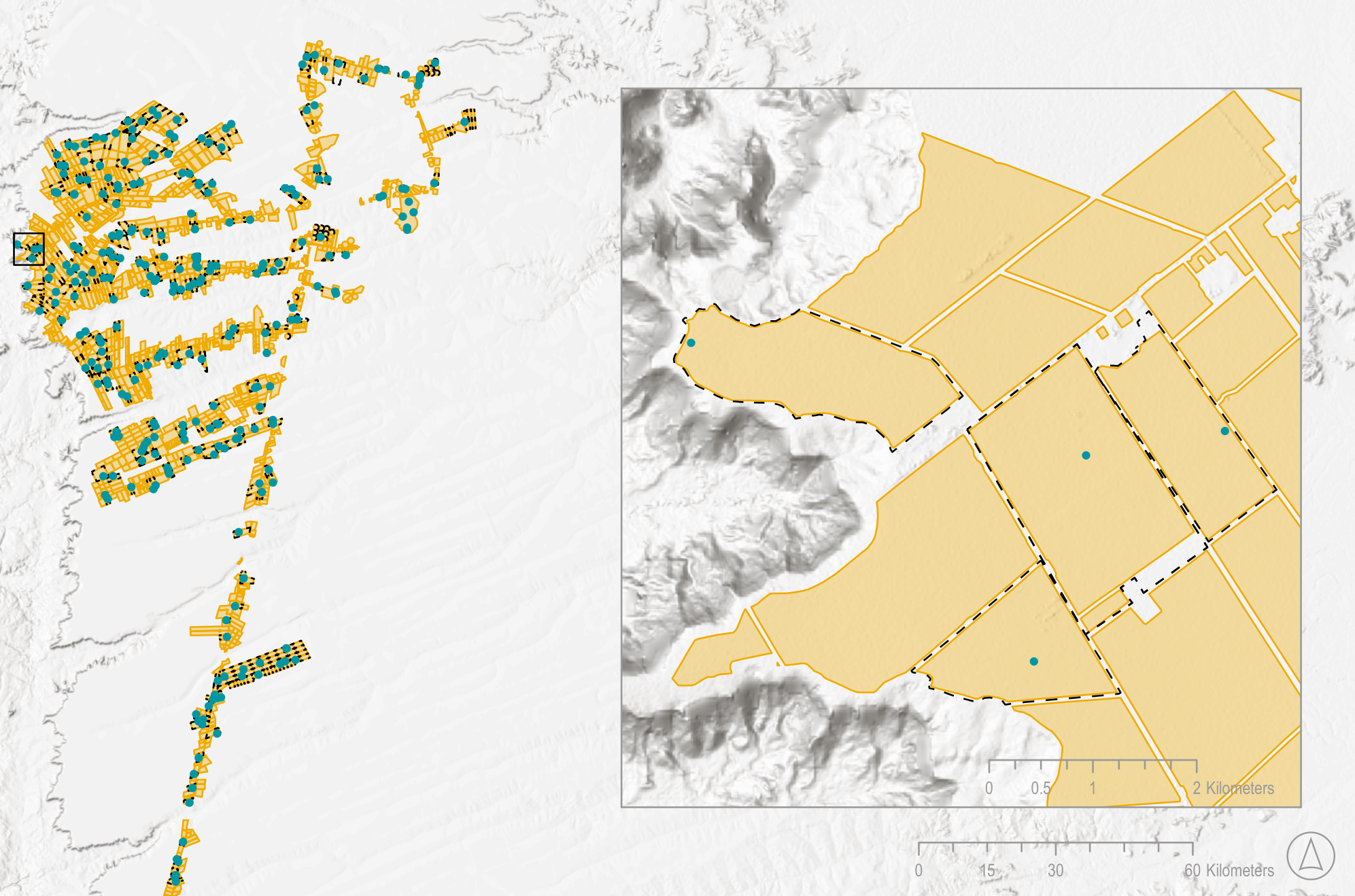
Manual annotations were compared with the Cerrado in-situ-informed ground-truth dataset of Oldoni et al. (2020), the 1,854 Brazilian fields included in the Fields of The World benchmark. Consistency is defined as similar overall size, object shape, and overlap. A single point was sampled at random within each field, rather than at its center, to avoid biasing annotators with morphology cues; 300 of the 1,854 points were then randomly selected, and annotators were asked whether a field boundary existed at each point and, if so, to draw it.
Figure 4. Manually annotated samples (dotted lines) compared to ground-truth samples (orange). Annotators drew a boundary, if a field was present, around random point locations (blue points) within randomly selected ground-truth fields, so not all ground-truth fields have a corresponding manual annotation. Ground truth: Oldoni et al. (2020).
Table 5. Metrics by field-size quartile: manual annotations vs. ground-truth boundaries
Quartile
Field size (ha)
IoU mean
IoU median
Centroid mean (m)
Centroid median (m)
BLR mean
BLR median
Q1
0.5 to 14.0
0.76
0.85
53.30
11.45
0.94
0.98
Q2
14.5 to 35.5
0.76
0.89
66.67
15.19
0.97
0.98
Q3
36.3 to 96.6
0.78
0.93
91.71
16.32
1.13
1.00
Q4
96.8 to 508.4
0.91
0.97
83.73
10.65
1.06
1.00
IoU = intersection over union; BLR = boundary length ratio. Source: Oldoni et al. (2020).
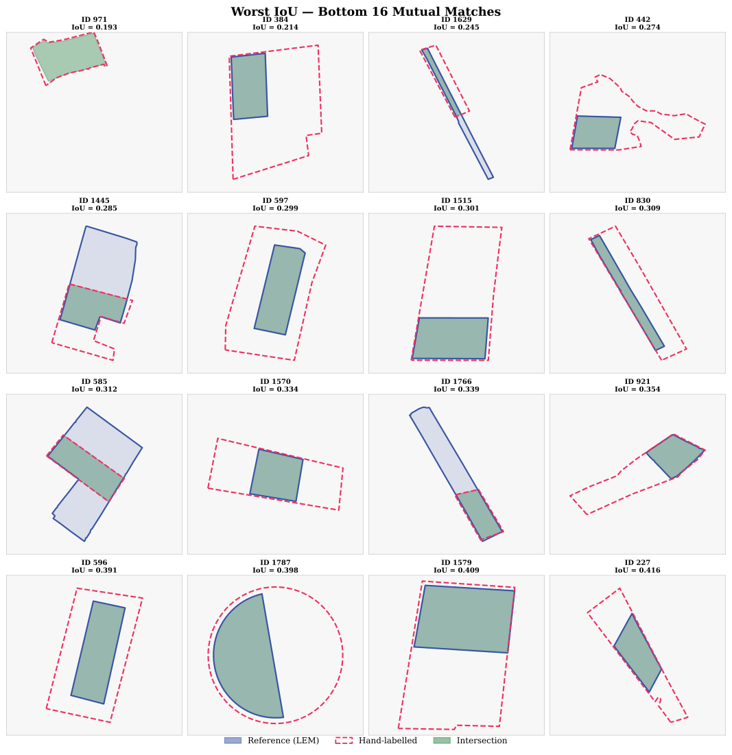
Agreement was highest for the largest fields (Q4: median IoU 0.97, median centroid distance 10.65 m). Smaller fields (Q1 and Q2) showed more variability (mean IoU 0.76), with a gap between mean and median indicating a subset of difficult cases. The elevated BLR in Q3 and Q4 suggests annotators traced slightly longer boundaries than the ground truth for larger fields, sometimes subdividing fields the ground truth treats as a single unit.
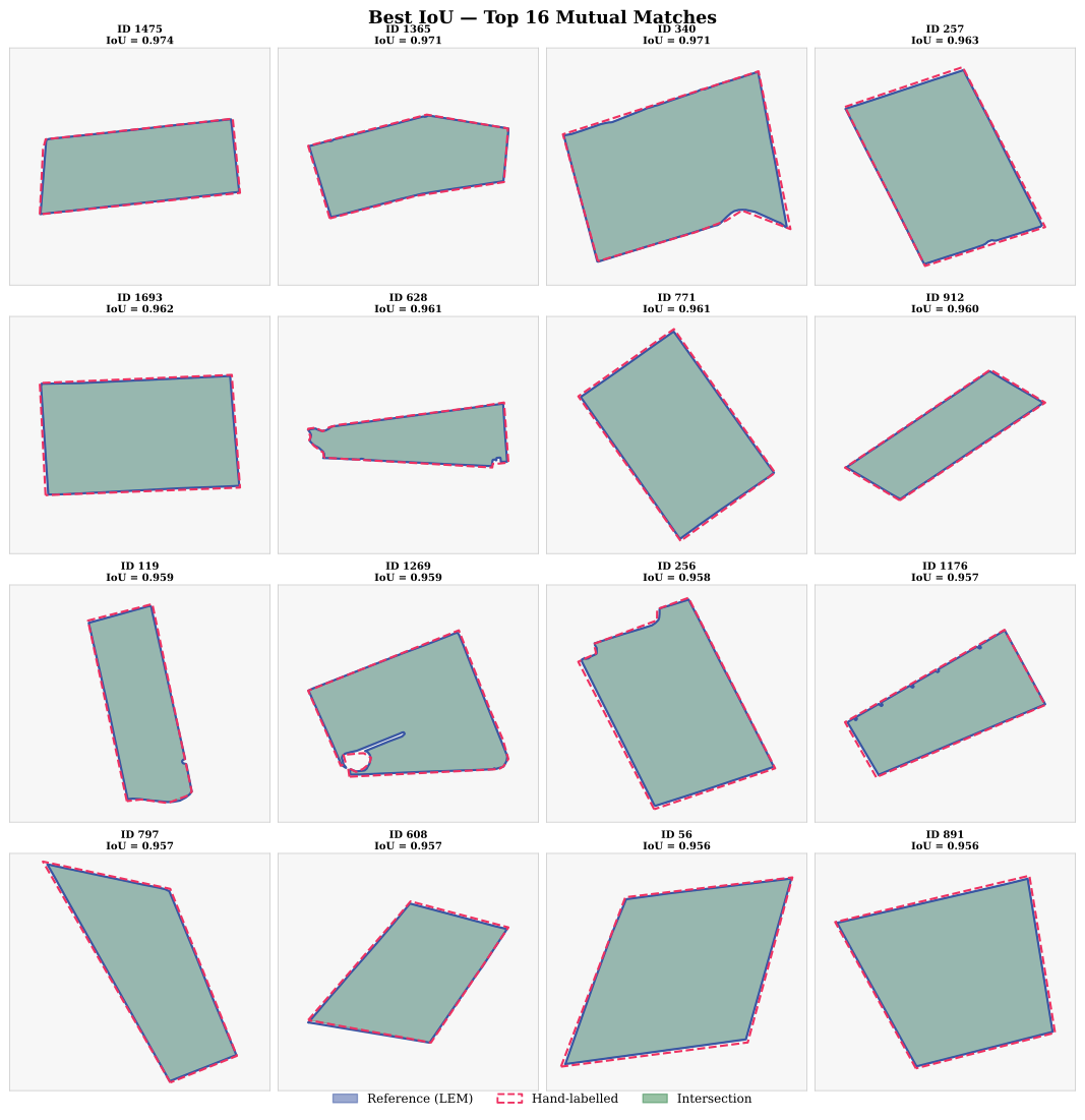
Figure 5. The 16 best IoU matches between manual annotations and ground truth.Figure 6. The 16 worst IoU matches between annotations and ground truth.
8.2 Inter-annotator agreement
When new annotators join the project, after completing their training they annotate a fixed calibration set: all fields they identify within 50 chips from one Sentinel-2 tile in Mato Grosso. These first annotations are compared against reference annotations drawn by the project data scientist who developed the criteria, calibrating new annotators to the project standard.
0.91
Median IoU between annotators and reference
0.80
Mean IoU across the four annotator pairs
0.02
Std. dev. of mean IoU across pairs
12.66 m
Median centroid distance across all pairs
Table 6. Each annotator vs. the reference annotator
Annotator pair
IoU mean
IoU median
Hausdorff mean
Hausdorff median
Centroid mean
Centroid median
BLR mean
BLR median
Reference vs. Annotator 1
0.78
0.91
209.28
42.86
81.01
12.09
1.03
1.00
Reference vs. Annotator 2
0.80
0.91
194.37
50.25
74.46
14.61
1.03
0.99
Reference vs. Annotator 3
0.81
0.91
181.07
47.19
68.24
13.26
1.00
0.99
Reference vs. Annotator 4
0.81
0.92
180.84
40.72
71.31
10.69
1.04
0.99
Mean
0.80
0.91
191.39
45.26
73.76
12.66
1.03
0.99
Std. dev.
0.02
0.01
13.50
4.28
5.46
1.67
0.02
0.01
Polygons were matched via spatial intersection and mutual best-IoU matching, using the reference annotator as the common comparison point. IoU = intersection over union; BLR = boundary length ratio.
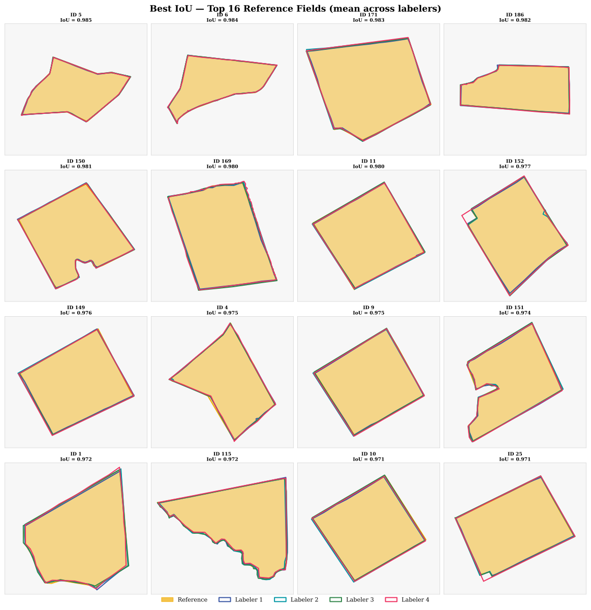
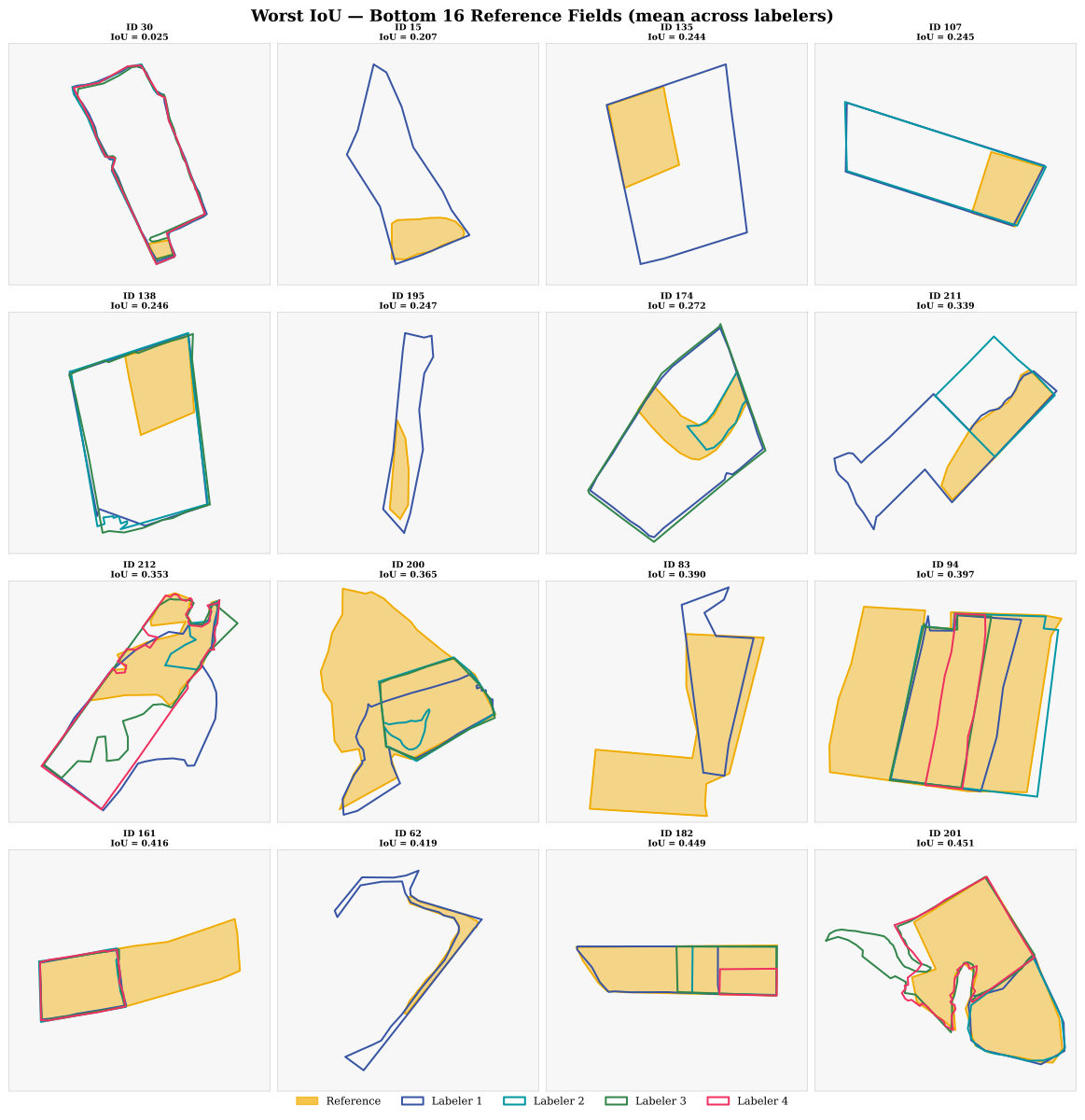
Total field counts ranged from 203 to 250 across annotators (reference: 215), differences of up to about 20 percent on a first attempt with only brief training. Even so, a median IoU of 0.91 represents near-perfect polygon overlap. For context, this is well above the 0.786 human inter-annotator benchmark reported for the Cityscapes dataset, and far above the mean IoU of 0.54 observed between expert medical-image annotators; industry standards broadly treat IoU above 0.8 as strong agreement. These results indicate that the annotation rules and guidelines produce consistent boundaries across annotators.
Figure 7. The 16 best IoU matches between the reference annotator and the annotation team, with near-perfect agreement.Figure 8. The 16 worst IoU matches between the reference annotator and the annotation team (Mato Grosso), illustrating differences in interpretation.